Welcome to the world of machine learning and deep learning. The main idea behind it is to train machine to learn from data so it can solve new cases even when the data changes. Besides, there are different types of learning tasks such as supervised learning(classification, regression, time series prediction) or unsupervised learning(clustering). Here, I need to touch on reinforcement learning in case i get confused in the future. So, there would be reward and penalty in reinforcement learning and the outcome is to choose best policy to maxmize rewards and avoid penaltie through learning from the past.
Table of Contents
Classification models
Outputs are categorical and inputs are anything. Goal is to select correct class(label) for new inputs.The simplest case is a choice between 1 and 0.
 Here, I need to address the difference between classification and regression . In the latter case, outputs are continnuous. But the goal is similar which is to predict outputs accurately for new inputs. We can use it to predict the price of astock in 6 months time.
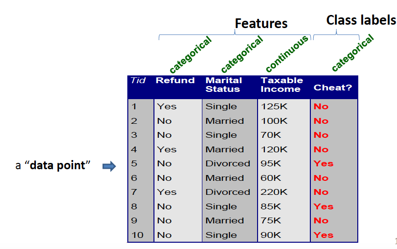
Before we dig into those complicated classification models, I want to list few examples where we can use those models and what we need to do before throwing bunch of stuff into our models. To start off, imagine predict whether a patient has cancer or not. Also, we can check if it is going to rain tomorrow based on temperature, humidity etc. The graph below is a vivid demonstration of inputs and outputs(matrix).
Here, I need to address the difference between classification and regression . In the latter case, outputs are continnuous. But the goal is similar which is to predict outputs accurately for new inputs. We can use it to predict the price of astock in 6 months time.
Before we dig into those complicated classification models, I want to list few examples where we can use those models and what we need to do before throwing bunch of stuff into our models. To start off, imagine predict whether a patient has cancer or not. Also, we can check if it is going to rain tomorrow based on temperature, humidity etc. The graph below is a vivid demonstration of inputs and outputs(matrix).
 Once we got a feature matrix, the following question is how to normalize features. This is because most of clssifiers calculate the distance between two points.
There are some ways to scale the range of a feature. The one I typically use is Min-max normalization
Okay, let me introduce you the first model: K-Nearest Neighbor(KNN). In one word, similar things are near each other and rely heavily on calculating distance. The implentation is shown below:
---
def knn(data, query, k, distance_fn, choice_fn):
    neighbor_distance = []
    for index, data_point in enumerate(data):
        distance = distance_fn(data_point[:-1],query)
        neighbor_distance.append((distance,index))
    sorted_neighbor_distance = sorted(neighbor_distance)[:k]
    k_nearest_labels = [reg_data[i][1] for distance, i in sorted_neighbor_distance]

    return k_nearest_labels, choice_fn(sorted_neigbor_distance)
---
---
def euclidean_distance(point1, point2):
    sum_squared_distance = 0
    for i in range(len(point1)):
        sum_squared_distance += math.pow(point1[i] - point2[i], 2)
    return math.sqrt(sum_squared_distance)
---
SOOOO,isn’t it perfect fit for recommendation system?? More details can be checked here.
As I mentioned before, in KNN, we often compute the following squared Euclidean distance between two data points x and z, d(x,z)=||x-z||**2. Here, we only needs to compute dot products between two data points and dot products between a datapoint and itself.
Next, I want to introduce Support Vector Machines(SVM) which is nothing more than a kernelized maximum-margin hyperplane classifier.
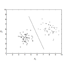
It is a linear classifier. The goal of it is to find the line which can “best” seperate two classes:
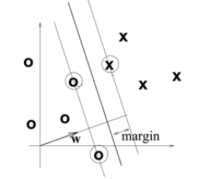
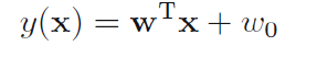 The vector w controls the decision boundary and w0 is called bias. We can assign an input vector x class C1 if y(x)>0 and to class C2 otherwise.
Thus SVM tries to make a decision boundary in such a way that the separation between the two classes is as wide as possible. Since somehow it would enlarge the feature space using kernels for accommodating a non-linear boundary between classes.
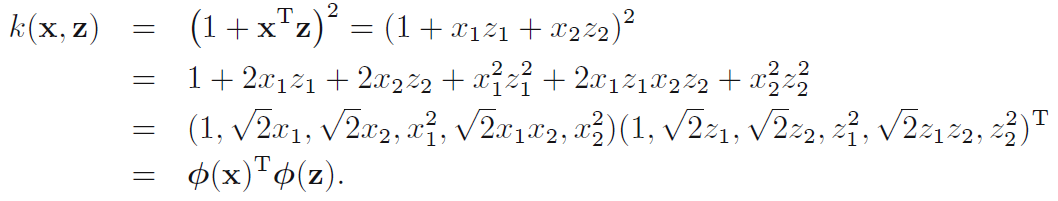
The key idea of kernal methods:
- Reduce an algorithm to one which depends only on dot products between data points
- Then replace the dot product with a kernal function k(x,z) in which k(x,z)=(1+xtz)2
An example of Kernal Trick. Start with 2-dimensional x=(x1,x2) and z=(x1,z2).
In order to understand the model more, I am gonna emphasize on following example with code written in python. Dataset, Details
import pandas as pd
import numpy as np
import matplotlib.pyplot as plt
from skelarn.preprocessing import LabelEncoder

cwd = 'path/mushroom.csv'
data = pd.read_csv(cwd)
data.head()
We notice that each feature is categorical and a letter is used to define a certain value(needed to be changed later).
Next, we want to see if our dataset is unbalanced. An unbalanced data set is when one class is much more present thant the other. Let us implement some sampling methods, like minority oversampling.
x = data['class'] ## class is defined into edible or posionous
ax = sns.countplot(x=x,data=data)
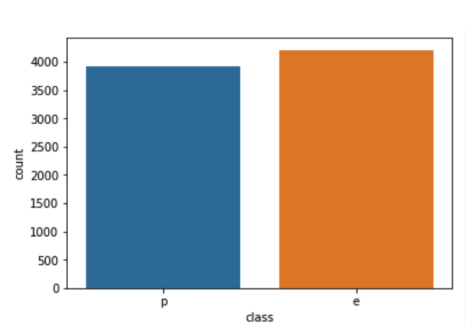
Perfect balanced data set. Now, we want to see how each feature affects the target. Specifically, I need to figure out this feature contributes more to edible class or another one.
def plot_data(hue,data):
   for i,col in enumerate(data.columns):
      plt.figure(i)
      sns.set(rc={'figure.figsize':(11.7,8.27)})
      ax = sns.countplot(x=data[col],hue=hue, data=data)
The hue will give a color code to the different classes.
hue  = data['class']
data2 = data.drop('class',1)
plot_data(hue,data2)
If you have confusion about how to use sns.countplot, Click Here
Now, let’s see if we have any missing values. Run this code below:
for col in data.columns:
    print("{}":"{}".format(col,data[col],isnull().sum()))
And we can see each column with the number of missing values. Next, we need to turn letters into numbers for modelling. To achieve this, we will use label encoding and one-hot encoding.
le = LabelEncoder()
data['class']=le.fit_transform(data['class'])
As a result, the content of class would be 0 and 1 instead of e and p. p is represented by 1 while e is represented by 0. This method comes with piority problem . Now that our data set contains only numerical data, we can now start our svm model and making preidctions. But before diving deep into modelling and making prediction, we need to split our data into a training set and test set.
from sklearn.model import train_test_split
X = data
y = data["class"]
X_train,X_test,y_train,y_test = train_test_split(X,y,test_size=0.3)
Here, y is simply the target(poisonous or edible). Sometimes, we will add parameter random_state to ensure that every time the code runs, the data set will be split identically.
from sklearn.svm import SVC
svclassifier = SVC(kernel = 'linear')
svcclassifier.fit(X_train,y_train)
Bingo, the simplest step of dealing with data set and you also learn how svm works.